Fundamental Analysis With Machine Learning in Python
By: Ari Silburt
Date: December 20th, 2017
The full code for this analysis can be found in my Machine Learning Repo.
If the EMH is false, money can be made by carefully selecting stocks. Surely you know of some person/entity who has boasted about analyzing market trends, carefully selecting a few stocks and earning huge profits. However, these cases by themselves don't falsify the EMH. For example, if I have 1,000 people each flip a coin 10 times, there will statistically be at least one person that flipped heads every single time. That person may think they are particularly amazing, when really it's just probability at play. Although random processes are used in many sectors of Finance today (e.g. Black-Scholes), it is still unclear whether stock prices really do evolve according to random walks.
Regardless of theory, it is an interesting exercise to see whether Machine Learning + Fundamental Analysis can be used to empirically predict future stock prices. Specifically, can we take all the stocks from the Wilshire 5000 index, get their stock prices and fundamental qualities at years $t$ and $t-1$, and accurately predict the stock price at year $t+1$? For concreteness, I will choose $t=2015$, but my code is generalizable to any $t$. I will also cast this problem as a classification problem instead of a regression problem. This means that if a stock increased between years $t$ and $t+1$ the machine learning algorithm should predict $1$, and $0$ otherwise. In contrast, casting this as a regression problem would mean I want to predict how much a stock increased or decreased between $t$ and $t+1$. As you can imagine, this is a much more difficult problem.
import pandas as pd
tickers = pd.read_csv('fundamental_analysis/wilshire5000.csv',delimiter=",")
tickers.head()
Next, we need the prices for each stock, which can be pretty easily obtained using the Yahoo! finance datareader, called through pandas (along with a fix, since Yahoo! decommissioned their historical data API). The following code gets the first couple stock prices for Agilent Technologies between Jan 1st-8th, 2015.
from pandas_datareader import data as pdr
import fix_yahoo_finance
pdr.get_data_yahoo(tickers['Symbol'][0], '2015-01-01', '2015-01-08')
Choosing $t=2015$, we will take the mean Adjusted Close prices from January 2015 ($P_t$) and January 2014 ($P_{t-1}$), and try to predict whether the mean Adjusted Close price in January 2016 ($P_{t+1}$) increased or decreased. That is, given $P_{t}$ and $P_{t-1}$ we will try to predict if $P_{t+1}/P_{t} > 1$. For the remainder of this post I define "winning" stocks to be those with $P_{t+1}/P_{t} > 1$ and "losing" stocks to be those with $P_{t+1}/P_{t} <= 1$.
Getting Financial Data
Next, we need to scrape all the relevant fundamental quantities for each stock and process them down into features. morningstar.com has an extensive list of "Key Ratios" and "Financials" for each stock. The image below shows an example for Agilent Technologies:
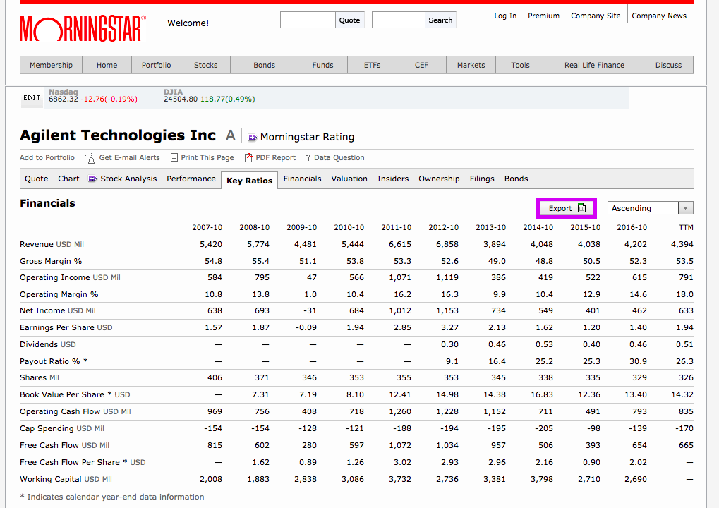
Highlighted in purple is the export button that muggles might use to manually download financial data for all 5000 stocks, one by one. However, there's a faster, more efficient way to get this info. We can scrape each stock's financial data into a csv file using the following code snippet:
from pattern.web import URL
for stock in tickers['Symbol']:
webpage = "http://financials.morningstar.com/ajax/exportKR2CSV.html?t=%s&culture=en-CA®ion=USA&order=asc&r=314562"%stock
url = URL(webpage)
f = open('%s_keyratios.csv'%stock, 'wb')
f.write(url.download())
f.close()
In the above code, the webpage variable was obtained by:
- Navigating to developer tools under Chrome web browser and clicking the network tab to monitor the ALL tab.
- Pressing the export button on the webpage for a single stock and find the corresponding url request sent in the ALL tab.
Preparing Data Arrays
Now comes the most difficult part. We need to process all the financial data into X and y data arrays that a machine learning algorithm can use. In principal it's not difficult, but there's a lot of cleaning and processing that has to happen like:
- Converting financial data that are cast in other currencies to USD (you'd think all stocks from the Wilshire 5000 would be in USD already...).
- Removing entire features that are sparsely filled.
- Fill missing values with median feature values for particular stocks.
- Taking Year-Over-Year (YOY) features whenever applicable.
- Generating new features that are not in morningstar like Debt/Equity, Price/Book, etc.
Performing all of the above yields a data array, X, that looks like:
X = pd.read_csv('fundamental_analysis/X.csv')
X.head()
The corresponding target output array, y, is an array of 0s and 1s corresponding to whether each stock is a loser or winner, respectively.
Machine Learning Time
An article by Forbes claimed that the average data scientist spends 60% of their time cleaning data, and this project is no exception. After a lot of scraping, cleaning and preparing, we are finally ready to do some machine learning. Here we will use XGBoost (eXtreme Gradient Boosted Decision Trees), a popular decision tree classifier.
We split our data into train and test sets so we can measure model performance on unseen test examples after training on the train set. In addition, we also scale our positive class by scale_pos_weight to offset any class imbalances, and tune the hyperparameters by performing a random grid search with cross validation:
import xgboost as xgb
from sklearn.model_selection import RandomizedSearchCV
from sklearn.model_selection import train_test_split

X_train, X_test, y_train, y_test = train_test_split(X, y, test_size=0.25, random_state=42)
scale_pos_weight = len(y_train[y_train==0])/float(len(y_train[y_train==1]))

model = xgb.XGBClassifier(scale_pos_weight=scale_pos_weight)
n_cv = 4        # of cross validation folds per randomized search
n_iter = 20     # of RandomizedSearchCV iterations
param_grid={
    'learning_rate': [0.1],
    'max_depth': [2,4,8,16],
    'min_child_weight': [0.05,0.1,0.2,0.5,1,3],
    'max_delta_step': [0,1,5,10],
    'colsample_bytree': [0.1,0.5,1],
    'gamma': [0,0.2,0.4,0.8],
    'n_estimators':[1000],
}

grid = RandomizedSearchCV(model, param_distributions=param_grid, n_iter=n_iter, cv=n_cv, scoring='roc_auc')
grid.fit(X_train,y_train)
Once our random grid search is complete we can take the best model and look at test predictions. In the plot below, the green histogram corresponds to stocks where $P_{t+1}/P_t >1$ (i.e. winners), the purple histogram corresponds to stocks where $P_{t+1}/P_t < 1$ (i.e. losers), and the x-axis shows the model-predicted probability that the stock is a winner.
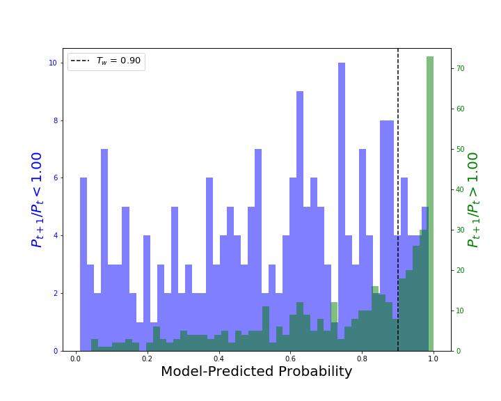
When a model outputs probabilities, there is no single "answer" but instead a range of answers that depends on your specific aims. Sometimes you want to recover as many positive cases as possible (at the cost of including many negative cases), while other times you want to avoid as many negative cases as possible (at the cost of rejecting most positive cases). The balance between these two scenarios is mediated through the precision and recall: $$ \rm{Precision} = \frac{T_p}{T_p + F_p}\\ \rm{Recall} = \frac{T_p}{T_p + F_n} $$ Here $T_p$ is the number of true positives (in our case: stocks correctly predicted by the model as winners), $F_p$ is the number of false positives (losing stocks incorrectly predicted by the model as winners), and $F_n$ is the number of false negatives (winning stocks incorrectly predicted by the model as losers). In order to make a firm classification we have to set a threshold $T_w$, i.e. all stocks with a model-predicted probability greater than $T_w$ are classified by the model as winners, while all others are classified by the model as losers. A dotted line corresponding to $T_w = 0.9$ is shown in the plot above, and for this case many winning stocks are correctly classified as winners but some losing stocks are also incorrectly classified as winners in the process. For $T_w=0.9$, $\rm{Precision} = 0.89$ and $\rm{Recall} = 0.40$.
In the context of Finance, a high precision and low recall is best. That is, we would prefer choosing only a few winning stocks but have high confidence in our predictions. Thus, we would likely set the classification threshold to $T_w=0.99$, giving us $\rm{Precision} = 1.0$ and $\rm{Recall} = 0.12$.
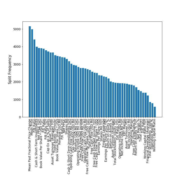
A really cool feature of XGBoost is the ability to rank feature importances. The plot below shows the relative importance of the top 20 features used by the model, ranked by split frequency (a.k.a. F-score):
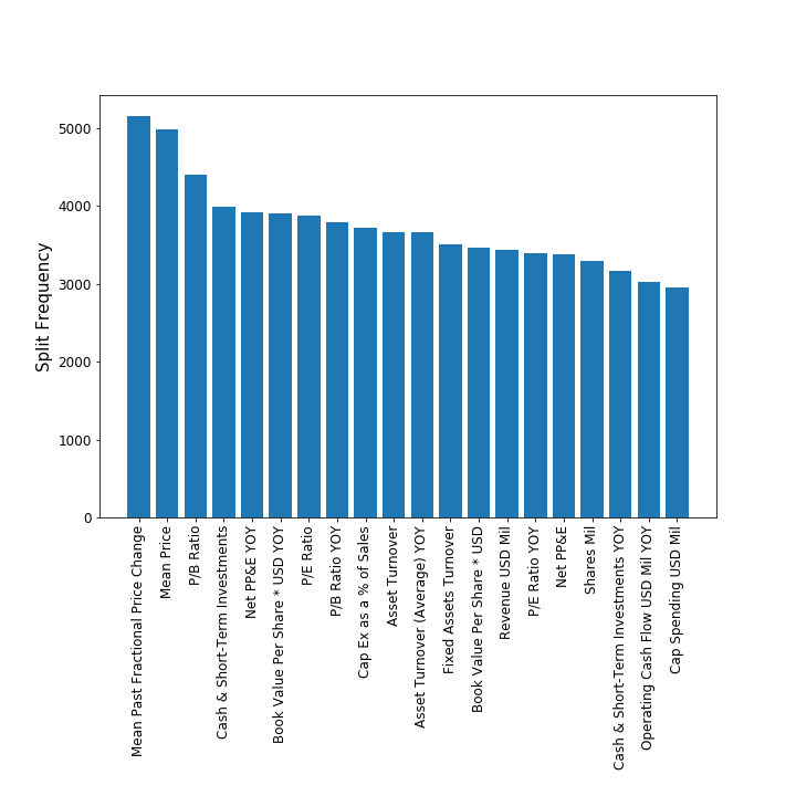
The top two features are the current price $P_{t}$ and the change in price $dP/dt$. This seems to support the concept of momentum in finance, i.e. stocks that have increased in the past are likely to increase in the near future. The third most important feature is the Price-to-book ratio, a well-known important financial ratio for measuring a company's profitability. Plotting all of the features below, we can see that some features like Working Capital Ratio, Operating Margin %, etc. are quite unimportant for predicting near-term profitability:
Summary and Improvements
In this post I walked through how to perform a fundamental analysis on a collection of stocks using machine learning in Python. In particular, I showed how to:
- Get price data for stocks in Python.
- Scrape financial data from Morningstar.com.
- Clean stock data and generate usable features.
- Train a machine learning algorithm to predict stock prices using financial data as input features.
- Analyze the results.
From here, one could start developing a trading strategy that would (hopefully) generate consistent positive returns over time. Looking at a few other years, sometimes the model doesn't do as well as hoped, while other times it does better. Further improvements could certainly be made to the above pipeline, like:
- Breaking the Wilshire 5000 index into individual sectors. Different sectors have different baseline standards, and mixing them together can confuse the model. For example, according to the Stern School of Business a Price/Book ratio of 1.5 is pretty good for a company in the banking sector but terrible for the broadcasting sector.
- Filter by marketcap - like sectors, different market caps (small, medium, large) will also have different baseline standards.
- Use a longer lookback time - Above we trained a model using only $t$ and $t-1$ to predict $t+1$, but one could easily extend the model to include $t-3$, $t-4$, ..., $t-X$ financial data.
- Cast the problem as a regression problem instead of classification. This is a more difficult but fruitful problem, since now you are trying to predict a value.
One thing to be wary of when implementing some of these improvements is that at some point your dataset will become too small to effectively train your model (as you chop the data up by sector, market cap, etc.). Machine learning in general requires a lot of data, and it was already perhaps pushing it already using only 5000 stocks to train the model (vs. say 50,000).
I hope you enjoyed this post analyzing stock prices using fundamental analysis and machine learning!
Helpful Links
Here are some helpful links used in making this blog post:
https://simply-python.com/2015/02/13/getting-historical-financial-statistics-of-stock-using-python/
http://stackoverflow.com/questions/40139537/scrape-yahoo-finance-financial-ratios
https://automatetheboringstuff.com/chapter11/
http://docs.python-guide.org/en/latest/scenarios/scrape/
https://www.boxcontrol.net/write-simple-currency-converter-in-python.html